ML Tooling
What is ML Tooling
ML Tooling is a toolbox developed to help put machine learning models into production
It also has a number of quality-of-life functions to avoid repeated code across projects
- Datasets
- Plotting
- Pandas-friendly transformers
- Logging
- Saving estimators
- Hyperparameter Search
Installation
pip install ml_tooling
Or
conda install ml_tooling
Ml-tooling ❤️ scikit-learn
ML Tooling is built on top of scikit-learn
This means that ML-Tooling is compatible with most Scikit-Learn workflows
We can use any estimator from Scikit-learn when creating our models
from ml_tooling import Model
from sklearn.ensemble import RandomForestClassifier

model = Model(RandomForestClassifier())
We can directly implement any Scikit-learn pipelines/transformers we want
from ml_tooling import Model
from sklearn.pipeline import Pipeline
from sklearn.preprocessing import StandardScaler
from sklearn.ensemble import RandomForestClassifier

>>> pipe = Pipeline([
...    ("scaler", StandardScaler),
...    ("classifier", RandomForestClassifier())
...])

>>> model = Model(pipe)
<Model: RandomForestClassifier>
(though to gain the full benefits, we should use ML-Tooling’s transformers)
Datasets
To use ML Tooling, we need the Model and we need a Dataset
The Dataset represents our access to data and tells ML Tooling how to load data for training and prediction
A Dataset must implement two method
load_training_data, which is expected to return a feature matrix and a target (X and y)load_prediction_data, which is expected to return a feature matrix and often accepts an ID of some kind to load data for that ID
As a general rule, we want everything in ML Tooling to be Pandas DataFrames
Implementing a Dataset
from  ml_tooling.data import Dataset
from sklearn.datasets import load_iris


class IrisDataset(Dataset):
    def load_training_data(self):
        """Implement how to load data when predicting"""
        # Load iris as dataframes
        iris_data = load_iris(as_frame=True)
        return iris_data.data, iris_data.target

    def load_prediction_data(self, idx):
        """Implement how to load data when predicting"""
        iris_data = load_iris(as_frame=True)
        return iris_data.data.iloc[[idx]]
We can now access the data
>>> iris_data = IrisDataset()
>>> iris_data.x
     sepal length (cm)  sepal width (cm)  petal length (cm)  petal width (cm)
0                  5.1               3.5                1.4               0.2
1                  4.9               3.0                1.4               0.2
2                  4.7               3.2                1.3               0.2
3                  4.6               3.1                1.5               0.2
4                  5.0               3.6                1.4               0.2
..                 ...               ...                ...               ...
145                6.7               3.0                5.2               2.3
146                6.3               2.5                5.0               1.9
147                6.5               3.0                5.2               2.0
148                6.2               3.4                5.4               2.3
149                5.9               3.0                5.1               1.8

[150 rows x 4 columns]
The first time x or y is accessed, ML Tooling calls load_training_data and then caches the result.
load_training_data is only ever called once.
Convenience Dataset
The two most common usecases is loading data from a file or loading from a database
ML Tooling ships with two Dataset implementations to help with these usecases
- FileDataset
- SQLDataset
FileDataset
Let’s dump our data to a parquet file, because csv’s are bad 😄
The parquet file will contain our data and target
import pandas as pd

# Make sure pyarrow is installed -> pip install pyarrow
pd.concat([load_iris(as_frame=True).data,
           load_iris(as_frame=True).target],
           axis=1).to_parquet("iris.parquet")
Our FileDataset will accept a filepath which we can use in our loading logic
class FileIrisData(FileDataset):
    def load_training_data(self):
        data = self.read_file()
        return data.drop(columns="target"), data.target

    def load_prediction_data(self, idx):
        data = self.read_file()
        return data.drop(columns="target").iloc[[idx]]
We can now point our FileDataset at the file we want to load
>>> file_data = FileIrisData("iris.parquet")
>>> file_data.x.head()
   sepal_length  sepal_width  petal_length  petal_width
0           5.1          3.5           1.4          0.2
1           4.9          3.0           1.4          0.2
2           4.7          3.2           1.3          0.2
3           4.6          3.1           1.5          0.2
4           5.0          3.6           1.4          0.2
SQLDataset
SQLDataset is used when connecting to a database to load data. Let’s create a local sqlite database
import pandas as pd
import sqlalchemy as sa

engine = sa.create_engine("sqlite:///iris.db")

(pd.concat([load_iris(as_frame=True).data,
            load_iris(as_frame=True).target],
            axis=1)
   # Make some more friendly column names
   .rename(columns=lambda x: x.rsplit(" ", 1)[0]
                              .replace(" ", "_")
   .to_sql("iris", engine)
   )
Creating a SQLDataset
from ml_tooling.data import SQLDataset

class SQLIrisData(SQLDataset):
    table = sa.Table(
        "iris",
        sa.MetaData(),
        sa.Column("index", sa.Integer, primary_key=True),
        sa.Column("sepal_length", sa.Float),
        sa.Column("sepal_width", sa.Float),
        sa.Column("petal_length", sa.Float),
        sa.Column("petal_width", sa.Float),
        sa.Column("target", sa.Integer)
    )
    def load_training_data(self, conn):
        select_statement = sa.select([self.table])
        data = pd.read_sql(select_statement,
                           conn,
                           index_col="index")
        return data.drop(columns="target"), data.target

    def load_prediction_data(self, idx, conn):
        select_statement = (
            sa.select([self.table.c.sepal_length,
                       self.table.c.sepal_width,
                       self.table.c.petal_length,
                       self.table.c.petal_width])
              .where(self.table.c.index == idx)
              )
        return pd.read_sql(select_statement, conn)
To use it, pass a conn string and what schema to use
(sqlite doesn’t have schemas, so we set it to None)
>>> sql_data = SQLIrisData(conn="sqlite:///iris.db", schema=None)
>>> sql_data.x.head()
       sepal_length  sepal_width  petal_length  petal_width
index
0               5.1          3.5           1.4          0.2
1               4.9          3.0           1.4          0.2
2               4.7          3.2           1.3          0.2
3               4.6          3.1           1.5          0.2
4               5.0          3.6           1.4          0.2
Copying data
One thing we can do with datasets, is to copy them between representations
(Make sure we delete our iris.parquet file)
import os
>>> os.remove('iris.parquet')
We can copy data from a SQLDataset to a FileDataset
new_file_data = sql_data.copy_to(file_data)
[13:24:55] - Copying data...
[13:24:55] - Dumping data from iris
[13:24:55] - Data dumped...
>>> new_file_data.x.head()
   index  sepal_length  sepal_width  petal_length  petal_width
0      0           5.1          3.5           1.4          0.2
1      1           4.9          3.0           1.4          0.2
2      2           4.7          3.2           1.3          0.2
3      3           4.6          3.1           1.5          0.2
4      4           5.0          3.6           1.4          0.2
Or from one SQLDataset to another if we need to move data between databases
>>> other_sql_data = SQLIrisData("sqlite:///other_iris.db",
                                 schema=None)
>>> sql_data.copy_to(other_sql_data)
[14:55:55] - Copying data...
[14:55:55] - Dumping data from iris
[14:55:55] - Data dumped...
[14:55:55] - Inserting data into iris
Exercise
- Go to https://www.kaggle.com/benroshan/factors-affecting-campus-placement
- Create a Kaggle account if you don’t have one
- Download the CSV
- Create a FileDataset based on this CSV
Plotting
ML Tooling comes with a number of plotting facilities to understand our data and models better
Dataset plotting
We can plot some basic information about our dataset that we implemented previously
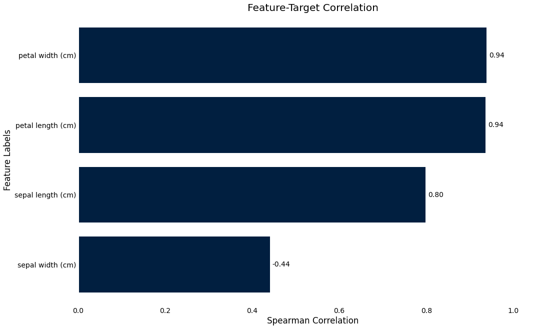
Target correlation
>>> iris_data.plot.target_correlation()
Missing data
This will show an overview of what data is missing in the dataset
>>> iris_data.plot.missing_data()
Result plots
To understand our model better, first we need to train a model. This will give us a Result object, which gives us access to
the plotting functionality.
from ml_tooling import Model
from sklearn.ensemble import RandomForestClassifier

>>> model = Model(RandomForestClassifier())
>>> result = model.score_estimator(iris_data)
[15:15:35] - Scoring estimator...
Note that all plots shown here have a plot_* counterpart to use if you want more finegrained control
When we train a model, we get back a Result object
>>> result
<Result RandomForestClassifier: {'accuracy': 0.89}>
The Result represents a scoring of the estimator and contains information about the metrics used for scoring and their results, as well as a number of convenience plotting functions
We can also do cross-validated scoring by passing a cv parameter
>>> result = model.score_estimator(iris_data, cv=10)
[15:23:17] - Scoring estimator...
[15:23:17] - Cross-validating...
>>> result
<Result RandomForestClassifier: {'accuracy': 0.96}>
We can now inspect the results by using the Results.plot accessor
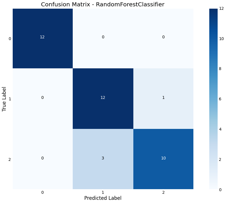
Confusion Matrix
We can plot a confusion matrix, with the option of normalizing
>>> result.plot.confusion_matrix(normalized=False)
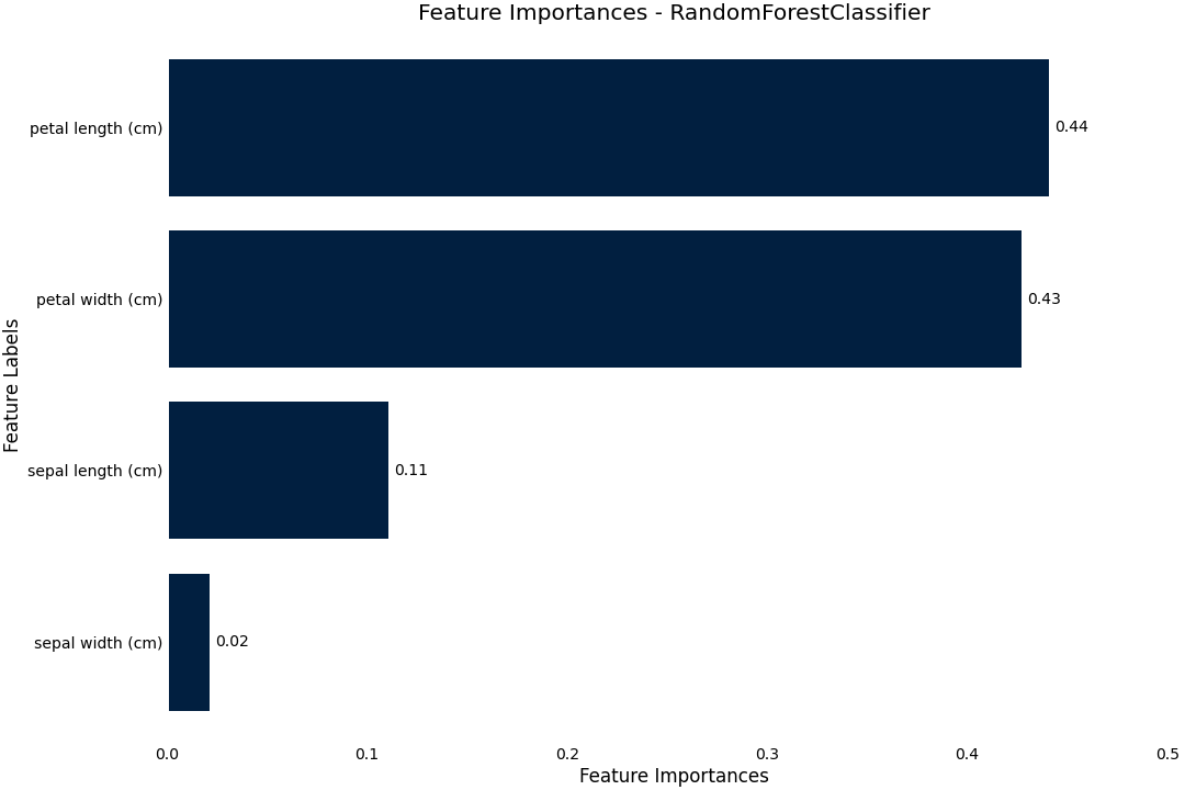
Feature Importance
We can plot feature importance based on either the model coefficients or the RandomForest feature_importance
>>> result.plot.feature_importance()
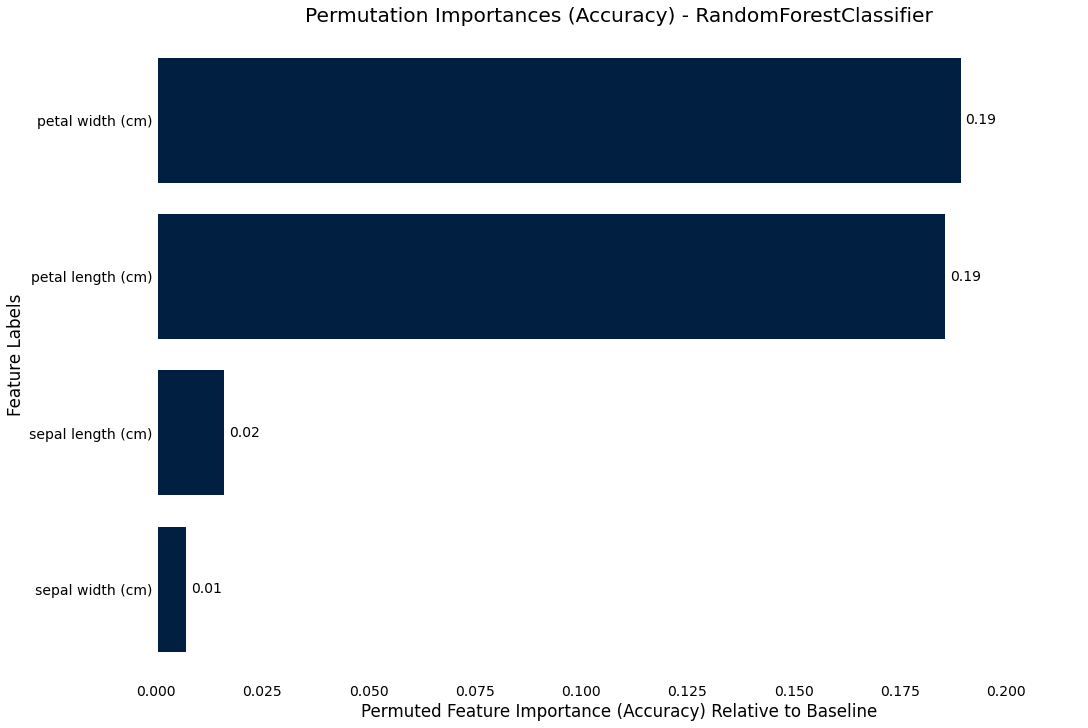
Permutation importance
We can also use the more precise, but more costly permutation_importance where we permute each column and compare the resultant score to
the baseline
>>> result.plot.permutation_importance()
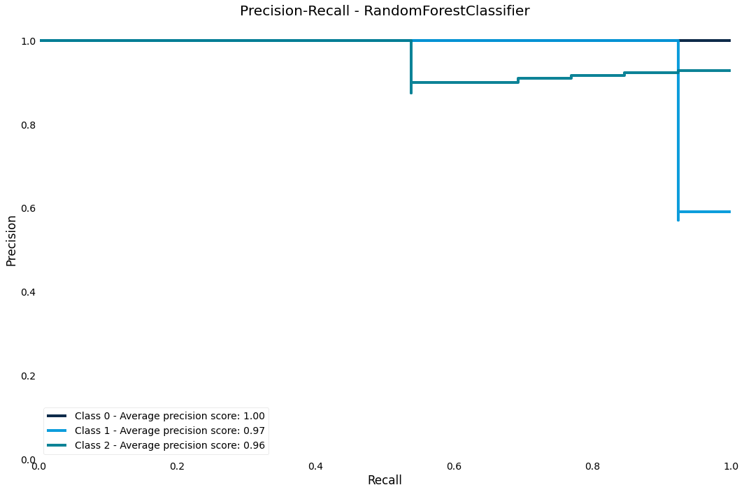
Precision-Recall curve
The precision-recall curve shows us how we are trading off precision and recall in the estimator across different thresholds
>>> result.plot.precision_recall()
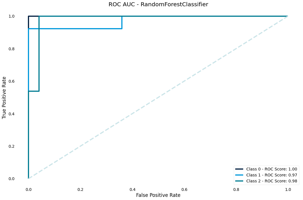
ROC AUC curve
The ROC curve is another classic performance plot for classification - we should generally always check the ROC of a classifier
>>> result.plot.roc_auc()
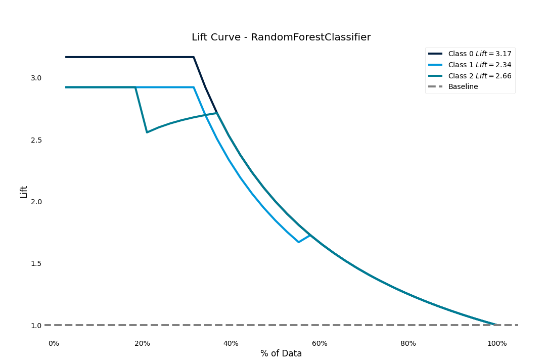
Lift score
The lift score will show us how much better our model is than random guessing
>>> result.plot.lift_curve()
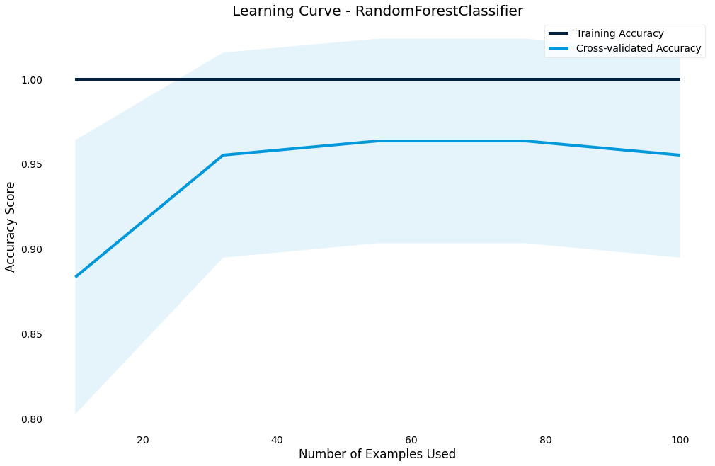
Learning curve
Another important chart is the learning curve - we use it to diagnose whether our model is under or overfitting and if we need to increase or decrease complexity
>>> result.plot.learning_curve()
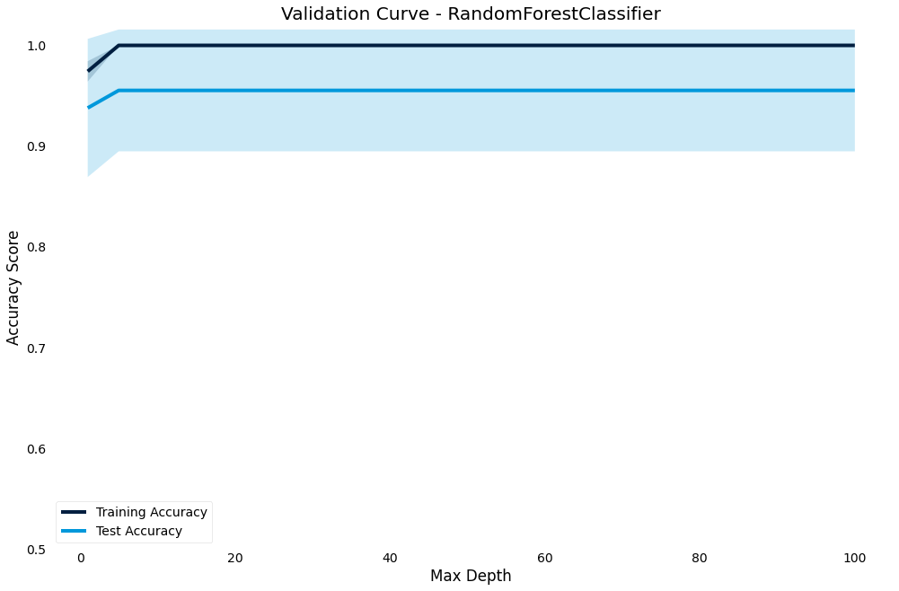
Validation curve
The validation curve lets you plot the performance of the model against a hyperparameter.
It shows effect of the hyperparameter on the model and gives an intuition for how the model responds to that parameter
>>> result.plot.validation_curve("max_depth",
                                 param_range=[1, 5, 10, 20, 30, 40, 60, 80, 100])
Regression
If we have a regression problem, the plots available will be different, although some will be available for both types
from ml_tooling.data import load_demo_dataset
from ml_tooling import Model
from sklearn.ensemble import RandomForestRegressor

>>> dataset = load_demo_dataset("boston")
>>> model = Model(RandomForestRegressor())
>>> result = model.score_estimator(dataset)
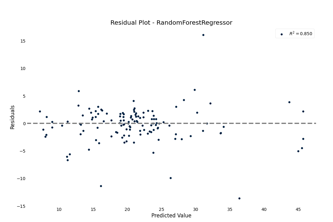
Residual plot
To check for goodness-of-fit, we can check the residual fit to verify that the residuals seem randomly distributed
>>> result.plot.residuals()
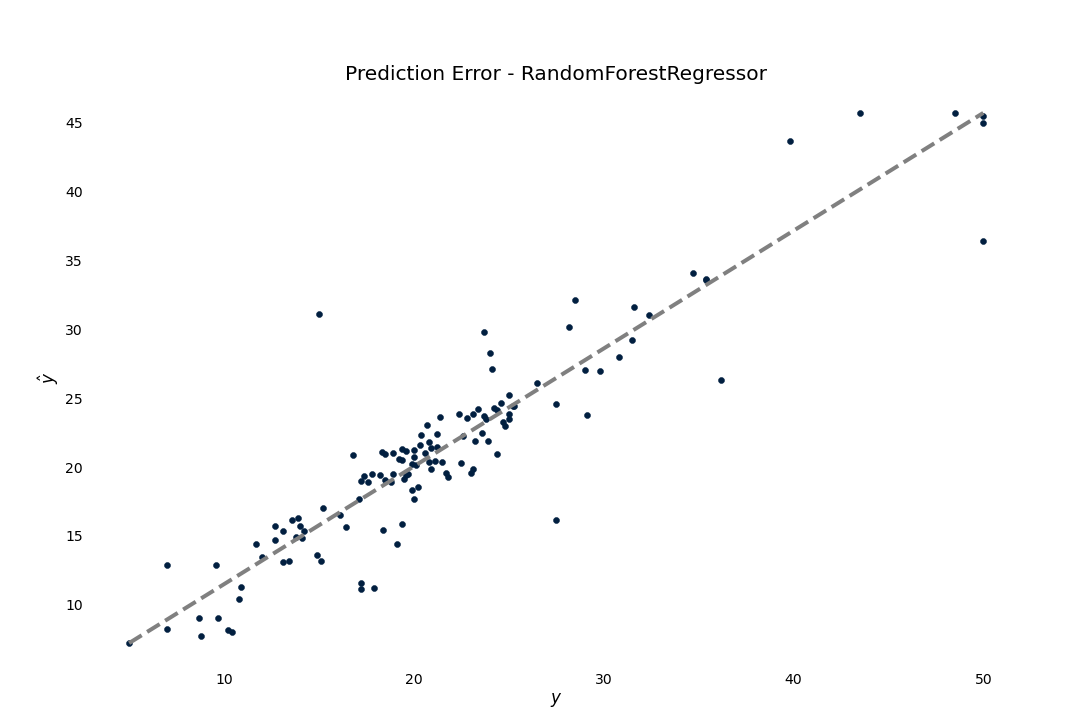
Prediction Error
We can also see how good the regression model is by plotting the predictions against the target
>>> result.plot.prediction_error()
Transformers
- Everything in ML Tooling is based around pandas
DataFrames - This lets us pass metadata such as column names to our functions and methods.
- Thus, we need to implement DataFrame-friendly transformers in ML-Tooling
The importance of Pipelines
- The
Pipelineis the foundation of building robust preprocessing in scikit-learn. - It lets us specify our entire data pipeline as a single object
- Additionally, scikit-learn makes sure to only learn attributes about your data when training, so that no accidental data leakage occurs.
An overview of transformers
- All ML Tooling transformers live in
ml_tooling.transformers - It’s simple to implement your own, and is considered part of the scikit-learn toolkit
- The documentation has plenty on the available transformers
A typical pipeline
We want to set up a Pipeline describing what features we want to use, how to preprocess them and join them together
Define our features
from ml_tooling.transformers import (
    Pipeline,
    DFFeatureUnion,
    Select,
    FillNA,
    ToCategorical,
    DFStandardScaler)

age = Pipeline([
    ("select", Select("age")),
    ("fillna", FillNA(strategy="mean", indicate_nan=True))
])

house_type = Pipeline([
    ("select", Select("house_type")),
    ("fillna", FillNA("missing", indicate_nan=True)),
    ("categorical", ToCategorical())
])

numerical = Pipeline([
    ("select", Select(["customer_since_days",
                       "car_probability",
                       "profitability"])),
    ("scale", DFStandardScaler())
])
Combine our features
feature_pipeline = DFFeatureUnion([
    ("age", age),
    ("housetype", house_type),
    ("numerical", numerical)
])

>>> feature_pipeline.fit_transform(train_x)
Define our Model
>>> model = Model(RandomForestClassifier(),
                  feature_pipeline=feature_pipeline)
Exercise
- Setup a pipeline for the FileDataset we made
- Train a model on the data
- Explore the plots
Logging
Log what our models do
- We can log the output of our models, so that we can keep track of what we have done previously
- ML Tooling can automatically keep track of the models we train if we turn on logging
>>> model = Model(RandomForestClassifier())
>>> with model.log("textclassifier"):
        model.score_estimator(dataset)
This will create a folder named “runs” with a yaml file inside
created_time: 2020-08-07 12:23:21.470576
estimator:
  // The entire pipeline definition...
- classname: RandomForestClassifier
  module: sklearn.ensemble._forest
  name: estimator
  params:
    // All the parameters...
estimator_path: null
git_hash: ''
metrics:
  accuracy: 0.8333333333333334
model_name: SchoolPlacement_RandomForestClassifier
versions:
  ml_tooling: 0.11.0
  pandas: 1.1.0
  sklearn: 0.23.1
We can reload the defined model from the saved yaml if we decide we want to retry a given model
>>> model = Model.from_yaml("./runs/placement/SchoolPlacement_RandomForestClassifier_130257_0.yaml")
Saving models
Storing your estimators
We can save our models as pickle files to reuse later or to put in production
Storage
We provide two Storage classes that let you store the model
- FileStorage
- ArtifactoryStorage
Create an instance of Storage and pass it to model.save_estimator
>>> storage = FileStorage("./my_models")
>>> model.save_estimator(storage)
[13:13:55] - Saved estimator to estimators/RandomForestClassifier_2020_08_07_13_13_55_137029.pkl
We can also log the saved estimator - this saves the estimator filepath to the log as well
>>> with model.log("classifier"):
...     model.save_estimator(fs)
ArtifactoryStorage
ArtifactoryStorage works similarly to FileStorage expect we need to instantiate it with the url, repo and authorization
storage = ArtifactoryStorage('http://artifactory.com',
                            repo='classifier_project',
                            api_key="MYAPIKEYHERE")
It can then be used just like FileStorage, but it will save and load estimators in Artifactory instead.
(Must have installed with the artifactory optional dependency - ml_tooling[artifactory])
Storing a production model
When you are ready to productionize your model we must
- Train the final estimator
- Save production estimator
# This will train a final model on all of X - no train-test split
>>> model.train_estimator()
>>> model.save_estimator(prod=True) # This will only work in a production package setting!
- A production estimator expects you to be working in a python package
- It looks for a setup.py/pyproject.toml file to establish the root of your project and puts the pickle file in the src folder
- If these don't exist then it will fail
- Make sure to include the pkl file in your package data before publishing your package!
Load production model
If you have installed an ML Tooling based package that has saved a production model correctly, we can load that model
model = Model.load_production_estimator("name_of_model_package")
This will load the production estimator from the python package
Searching
ML Tooling implements three hyperparameter search options
- Gridsearch
- Randomsearch
- Bayesiansearh
Gridsearch
Classic gridsearch
>>> param_grid = {"estimator__max_depth": [1, 2, 4, 8, 16, 32, 64]}
>>> best_model, results = model.gridsearch(dataset,
                                           param_grid=param_grid)
We use gridsearch to explore the hyperparameter space systematically
- Focus on one hyperparameter at a time
- Start with a wide range and narrow it down
Randomsearch
- Randomsearch is used to cover a larger hyperparameter space with the same “budget”
- This is often a good first pass if we have no prior knowledge of where to search
To use, we specify distributions to sample from using Space objects from skopt
from ml_tooling.search import Integer

>>> param_distributions={"estimator__max_depth": Integer(1, 200)}
>>> best_estimator, results = model.randomsearch(
                          dataset,
                          param_distributions=param_distributions)
By default, we run 10 trials, but can change that with the n_iter parameter
Bayesiansearch
- Often more effective than Randomsearch, but can be more expensive since it cannot be parallelized
- Uses the results of the previous result to guide the choice of the next hyperparameter from the distributions
>>> param_distributions = {"estimator_max_depth": Integer(1, 200)}
>>> best_estimator, results = model.bayesiansearch(
                              dataset,
                              param_distributions=param_distributions)
Like randomsearch, bayesiansearch runs 10 trials by default
ResultGroups
For all the searches we get back a ResultGroup- a container for Results.
best_estimator, results = model.bayesiansearch(dataset,
                          param_distributions={"estimator__max_depth": Integer(1, 200)},
                          metrics=["accuracy", "roc_auc"],
                          n_iter=2)
>>> results
ResultGroup(results=[
    <Result RandomForestClassifier: {'accuracy': 0.85, 'roc_auc': 0.93}>,
    <Result RandomForestClassifier: {'accuracy': 0.84, 'roc_auc': 0.94}>])
The ResultGroup sorts by the first metric passed, but we can change the sorting, either by changing the order passed or by calling sort
>>> result.sort(by="roc_auc")
ResultGroup(results=[
    <Result RandomForestClassifier: {'accuracy': 0.84, 'roc_auc': 0.94}>,
    <Result RandomForestClassifier: {'accuracy': 0.85, 'roc_auc': 0.93}>])
Attribute access is delegated to the first result - otherwise we have to index into the ResultGroup
>>> results.metrics # We get the first result's metrics
Metrics(metrics=[
        Metric(name='accuracy', score=0.8444852941176471),
        Metric(name='roc_auc', score=0.9356060606060606)])
>>> results[1].metrics
Metrics(metrics=[
        Metric(name='accuracy', score=0.8511029411764707),
        Metric(name='roc_auc', score=0.931060606060606)])
Remember, we can log searches too - we get one log per model trained
param_distributions = {"estimator__max_depth": Integer(1, 200)}

with model.log("search"):
    best_estimator, results = model.bayesiansearch(
                          dataset,
                          param_distributions=param_distributions,
                          metrics=["accuracy", "roc_auc"],
                          n_iter=2)
Final Assignment
Build the best model you can on the data
- Try some different hyperparameter searches
- Log some results
- Save the best estimators
Additional Resources
Issues
If any issues arise, make sure to file an issue here